
Imagine you join a new project with a clear goal, improve ClickHouse performance, so our biggest customers can run their queries in a reasonable amount of time. This is something you’ve done lots of times before. You ask for the most expensive query since it’s usually the one that will have the most impact and a few low-hanging fruit improvements. You run it and it takes more than a minute to complete.
1 row in set. Elapsed: 85.715 sec. Processed 1.96 billion rows, 198.69 GB
Peak memory usage: 23.05 GiB.
The query is one of the twelve being run in parallel, each computing its own metric or sparkline. And they are in the first screen a client lands on when accessing the application. Imagine a client looking at a spinner for at least a couple of minutes right after logging in.
This is a note on all the changes, learnings, and optimizations we’ve made during the last four months to bring that query to sub-second latency. Changes were simple and incremental. None of them was a clever trick, just basic improvements compounding on each other.
ReplacingMergeTree Is No Fun
The setup is simple, events get written to a ClickHouse table directly from Kafka. Events are mutable, any event at any given point in time can be updated or deleted1. So, events changing past history are being received at similar or even faster rates than new events. Exactly what a database based on immutable storage is not for. We are forced to use ReplacingMergeTree engine and make heavy use of FINAL, that’s where most of the time goes.
On top of that, there are a few metrics that require going through the entire history of a client’s events to be computed. History that is always increasing since they keep their activity and generate events every day. For this reason, some numbers in this post may vary. An optimization that took a query from 200GB to 150GB could later be seen reading 210GB due to the amount of data received between one optimization and the next2.
The Weird Partition Key
The table was originally partitioned by month:
PARTITION BY toYYYYMM(event_created_at)This is the obvious choice, but the wrong one in many ways for this case.
Events come in batches, and those batches impact any point in time. A single batch will contain events from multiple months, writing a lot of files per insert and causing the usual snowball effect: increasing the number of files real-time queries have to read, adding pressure to merges, etc.
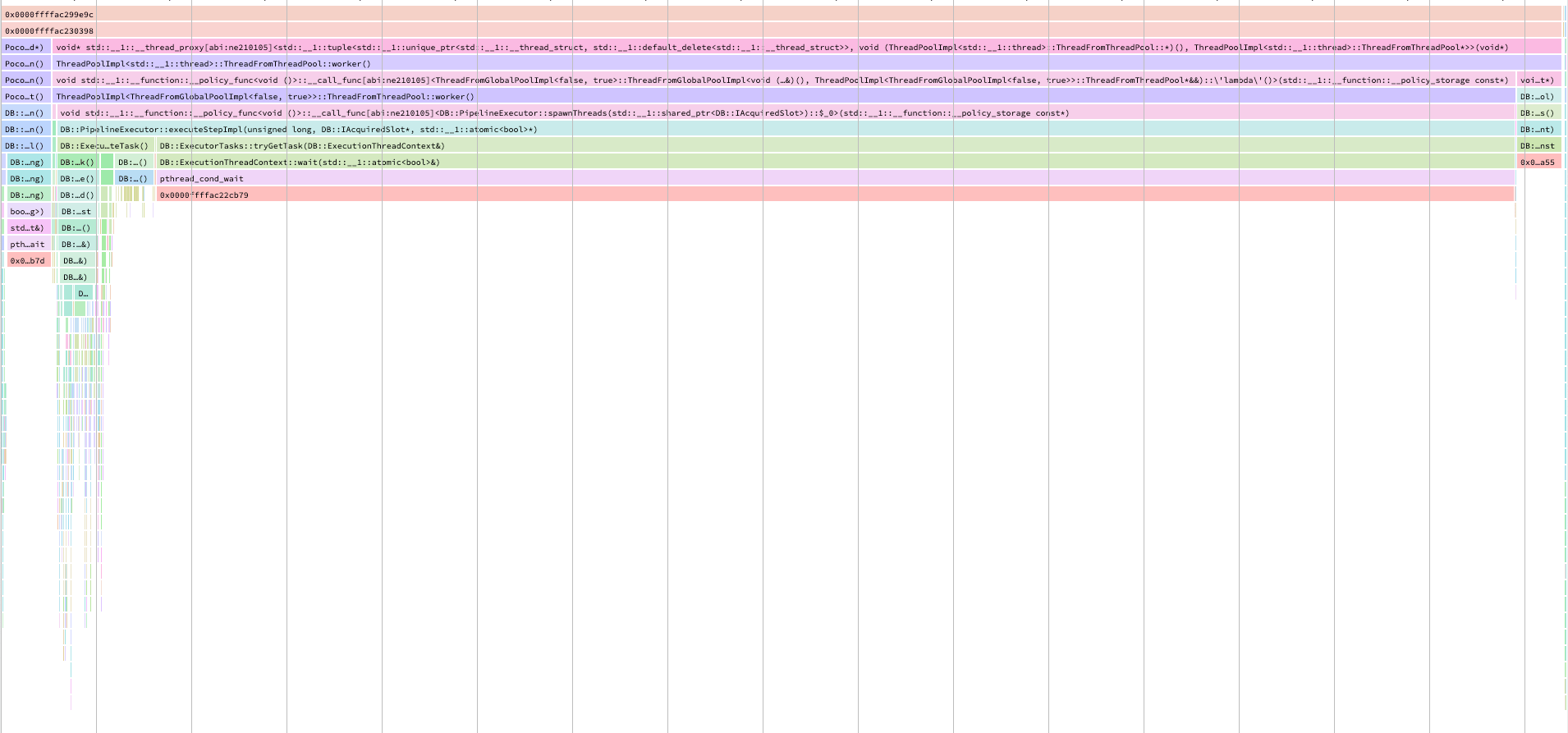
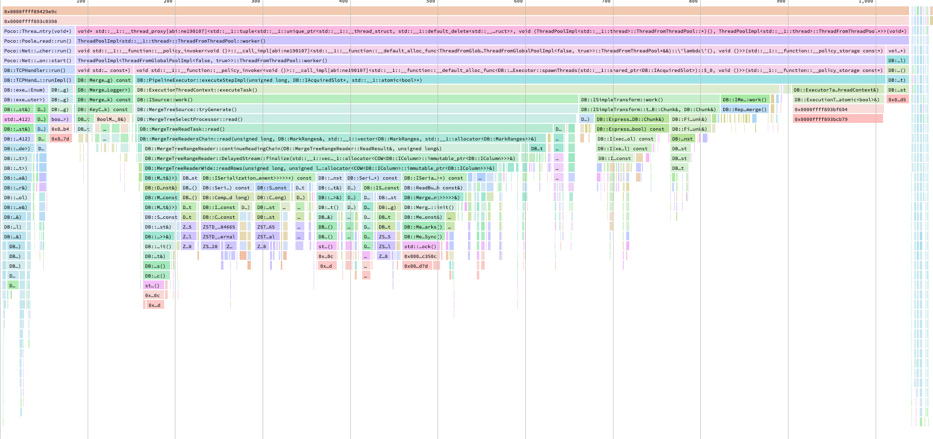
Also, FINAL merges rows together, and its parallelism depends a lot on how keys are distributed across partitions and how they overlap, the worst case scenario is a single thread doing the final merge and taking a lot of time. Partitioning by time means that a client’s events are spread across every partition in the table, so ClickHouse has to spend a considerable amount of time building the pipeline and splitting ranges to reduce intersections.
An example of the performance impact of this partitioning causing FINAL to be performed by a single thread:
To solve both issues while gaining a bit of performance, we applied the following partitioning strategy:
PARTITION BY (client_customer_id % 36)Note that client_customer_id is not our client’s id but our client’s client id, we don’t use this column in our queries. The strategy is counterintuitive3 but it works well for our use case:
- Keeps insert performance under control by “only” creating 36 parts per insert
- Partitions are equally distributed. There are no huge partitions containing whale clients and slowing down queries for every client landing in the same partition
- Ensures
FINALparallelism without requiring ClickHouse to compute ranges intersections. Which means that we can disablesplit_parts_ranges_into_intersecting_and_non_intersecting_finalandsplit_intersecting_parts_ranges_into_layers_finalsaving a few extra seconds on the data pipeline building step - We give up partition pruning entirely, since we never filter by
client_customer_id. There is a cost, but not for metrics that have to read a client’s full history anyway. Partitioning by month was not pruning anything either. And as mentioned above, we gain a lot in parallelism
Order By Slightly Changed
While checking how every event_type contributes to each metric, we discovered that a few of them didn’t contribute but we were still reading and processing them. They were ~16% of the rows on the table. Not a huge difference but an obvious change that could improve query performance.
Promoting event_type to an earlier position is not an ALTER. The sorting key is fixed when the table is created, so this meant a new table and a full rewrite. Behaviour stayed the same, since event_type was already in the key and only its position moved, so ReplacingMergeTree still collapses exactly the rows it collapsed before. After the change, we saw a significant improvement in query performance:
Before4
1 row in set. Elapsed: 13.43 sec. Processed 256.67 million rows, 18.82 GiB
Peak memory usage: 18.78 GiB.
After
1 row in set. Elapsed: 11.44 sec. Processed 237.86 million rows, 15.67 GiB
Peak memory usage: 14.04 GiB.
The query latency improved by ~15% while reading ~7% fewer rows. That explains why we don’t see the full ~16%: the sorting key filters out granules, and if a granule contains even one row of an event_type we are interested in, we have to read the remaining rows from that granule.
Removing an Expensive Join
The query had a few expensive joins, almost all of them behind a trick that let us skip the real table without removing the join. The right side is a subquery gated by a parameter, so when the branch isn’t needed the filter is false and it returns nothing:
ANY LEFT JOIN (
    SELECT ...
    FROM table_2
    WHERE {has_currency:Boolean} = 1 AND ...
) USING ...
Executing that costs a few milliseconds, parsing and planning it a few more. That’s what the templating section is about.
There was a join though that was being performed against a real table on every single call. The join was simply retrieving a couple of fields used to compute some intermediate values used for the metrics.
ANY LEFT JOIN (
    SELECT
        client_id,
        internal_id,
        latest_a_field,
        latest_another_field
    FROM table_derived_from_original_table FINAL
    PREWHERE client_id IN {client_ids:Array(UInt64)}
) USING client_id, internal_id
A second FINAL on a table derived from the original one to compute the latest values of the two fields we were interested in. ClickHouse builds the hash table for the right side and puts it in memory, the join is relatively fast but the cost is not only reading but also in memory footprint.
The fix was easier than it seems. The intermediate column computed with these two values could be precomputed at application level and sent as part of the event. The queries are now simpler and the join can be removed entirely.
1 row in set. Elapsed: 2.46 sec. Processed 49.86 million rows, 5.60 GiB
Peak memory usage: 1.09 GiB
Memory went down almost 13x, and query time improved by almost 5x.
Reading Fewer Columns
We have seen how precomputing a column at application level can save us a lot of memory and CPU. Why should we stop there?
Turns out that some of the metrics, especially the ones that require to read full client’s history, were using 9 columns. This is not a big deal with row-based databases but ClickHouse is columnar and reading a large number of columns means accessing extra data that could be avoided otherwise.
After precomputing the metrics contribution for each row at application level5, the impact was clear.
1 row in set. Elapsed: 1.38 s. Processed 49.69 million rows, 3.46 GiB
Peak memory usage: 582.40 MiB
The 9 columns came to roughly 38 bytes per row. Replacing them with an 8-byte column saves 1.5GB of reads on its own. Add the extra files you avoid reading, indices and marks, plus the seeks you save. And you get another ~2x improvement.
Templating
At this point, we have managed to go from 13.43s to 1.38s, that’s almost a 10x improvement by just compounding optimizations that we managed to apply in a few weeks. During the process, we have observed a few things that need to be addressed with a more aggressive approach.
One of the biggest bottlenecks we identified was related to how queries are being executed. We were using nested ClickHouse parameterized views, three levels deep generating huge queries that were re-parsed and re-planned on every single request. Those views were passing parameters and rendering some optional branches like the joins mentioned above. No matter what we tried, the branches were still there consuming CPU even if it was not being used.
Measuring the impact was easy. Building a minimal version of the query and running it against a client without data. Execution is almost zero, so everything left is parse, AST, and pipeline building6:
| Metric | Original | Simplified | Delta |
|---|---|---|---|
| metric_1 | 0.448s | 0.029s | 420ms |
| metric_2 | 1.345s | 0.051s | 1.3s |
420ms of fixed overhead on a query whose average execution time was 740ms. More than half of the time was spent on preparing the query.
So we replaced the views with flat query templates. dbt compiles each metric into a single self-contained statement (from the same macros that build the parameterized views, so there’s one source of truth) leaving second-stage markers with bracket delimiters, which pass through dbt’s own curly-brace Jinja untouched:
SELECT
    [% if has_currency %]
        {currency:String} as display_currency,
        coalesce(nullIf(exchange_rate, 0), 1)
    [% else %]
        'USD' as display_currency,
        1
    [% endif %] AS exchange_rate,
    money_field_in_usd * exchange_rate as money_field_in_display_currency
FROM original_table FINAL
PREWHERE client_id IN {client_ids:Array(UInt64)}
[% if has_currency %]
ANY LEFT JOIN (
    SELECT date, exchange_rate
    FROM exchange_rates PREWHERE currency = {currency:String}
) USING date
[% endif %]
The application renders the Jinja template (with the bracket delimiters) per request. Rendered queries are a few KB instead of 20+ KB. As you can see in the example, with no currency, the exchange-rate join doesn’t exist in the query at all.
The A/B result tagged through log_comment in system.query_log:
| Metric | Approach | Avg ms | p99 ms | Total CPU (s) |
|---|---|---|---|---|
| metric_1 | template | 233 | 626 | 44,897 |
| metric_1 | view | 735 | 1,355 | 67,199 |
| metric_2 | template | 448 | 1,290 | 58,403 |
| metric_2 | view | 1,835 | 2,940 | 100,885 |
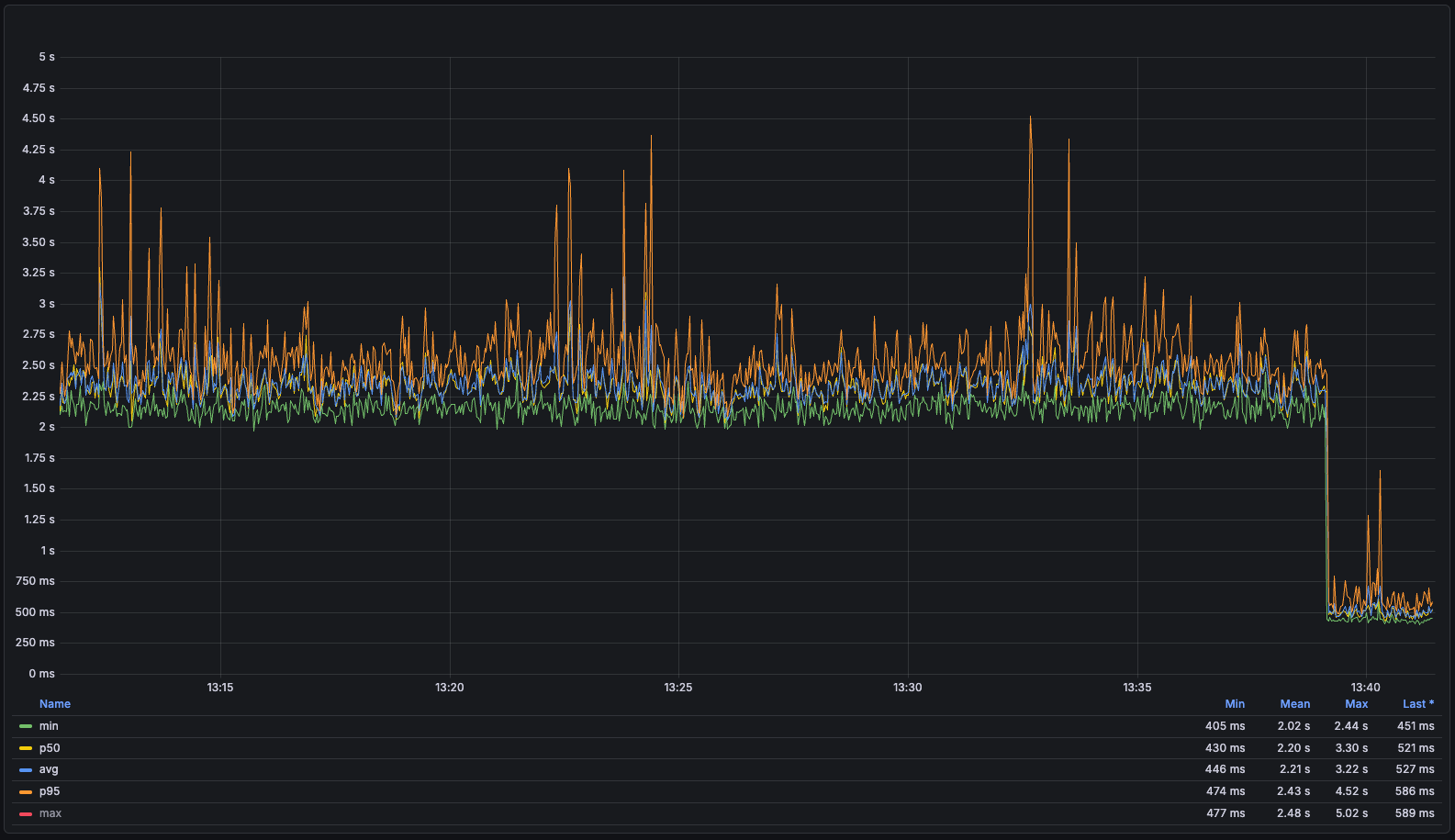
Results from another query, way more impressive in Grafana:
Of course, this comes at a price. The templates have to be compiled and rendered on the application server. The initial approach was caching the compiled templates in memory, but this was not enough due to the thousands of servers we run and how often they get restarted due to deployments. The heavy templates were taking over 300ms. We added an extra cache layer, moving the compiled bytecode to memcached. If the template is not found in memory, we try to fetch it from memcached, and if it’s not found there, we compile it on the fly.
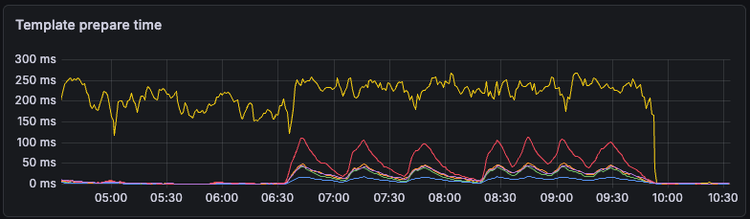
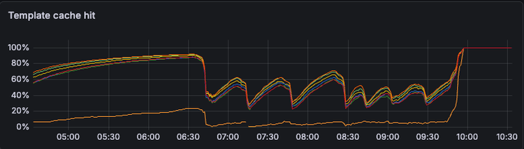
Compilation time can be considered roughly zero.
Those queries run roughly 2.4 million times a week, so small per-query savings keep compounding into something the cluster can feel.
Aggressive Merges
The templating managed to cut down a constant overhead we had in all our queries. The impact was limited though, and the improvement is relatively small for queries that are still reading a lot of data.
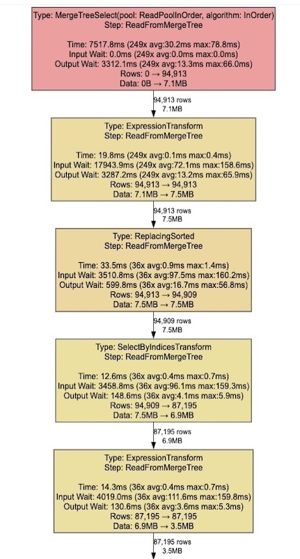
Now it’s time to start reading less data. The easiest way I have found is to analyze the information in system.processors_profile_log. We even have a tool to plot the results. See how the query we are trying to optimize looks like:
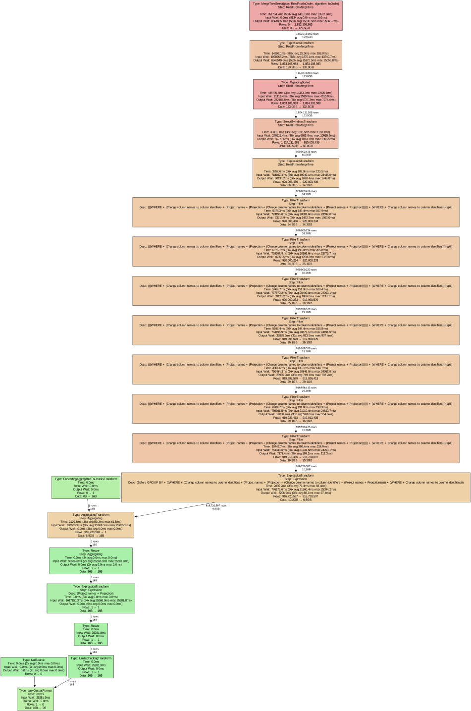
Since we are trying to make this query to read less data, we can focus on the first four or five stages of the pipeline. These are the stages responsible for reading data and apply the FINAL deduplication. Everything that happens after that is other filters, aggregations, etc. and we are not interested in that now.
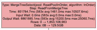
PREWHERE already applied.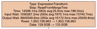
toDate(...))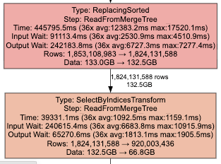
FINAL dedupes, then indices halve the rows.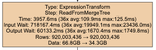
FINAL: 66.8 GB to 34.3 GB.A few important things to note:
- We read 130GB of data but only 35GB are relevant for the computation
- There is already a 2x duplication in our tables (1.8B rows → 920M rows)
- Columns from the sorting key being read only to apply the
FINALrepresent 30GB of the 60GB. If we take into account the 2x duplication, these columns represent 60GB of the 130GB read from disk.
A ReplacingMergeTree is only as clean as its merges, and somehow merges were stuck:
Totals:
   ┌─partition─┬─parts─┬──parts_+30_gb──┬──perc─┬─bytes────┐
1. │           │   534 │             32 │ 50.73 │ 2.12 TiB │
   └───────────┴───────┴────────────────┴───────┴──────────┘
32 of 36 partitions contained a single part larger than 30GB holding about 50% of the partition rows. And looks like our merges limit (max_bytes_to_merge_at_max_space_in_pool) was set at 50GB. Those parts were never going to get merged with anything again, so every duplicate that landed next to them is kept forever.
Two settings changed here:
max_bytes_to_merge_at_max_space_in_poolwas raised from 50GB to 100GB, so parts larger than 30GB that had never been merged would have a chance againmin_age_to_force_merge_secondswas set to 86400 (24 hours), so parts older than 24 hours were merged
The first one did nothing, probably because the merge selector filters merge input size by how much room is left in the merge pool. Also, max_bytes_to_merge_* applies to the input, not the result. Because this is a ReplacingMergeTree, deduplication makes the output smaller than the sum of its parts (i.e., a 55.9 GiB input produces a 40.69 GiB part)
The second one did the trick, parts older than 24 hours were merged regularly. Back on production data, the table got optimized:
| Value | Before Merges | After Merges |
|---|---|---|
| Parts | 534 | 378 |
| Table Size | 2.12 TiB | 1.55 TiB |
| Biggest Client Query Time | 14s | 5.5s |
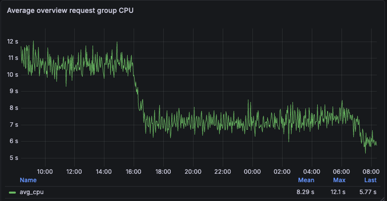
FINAL gets cheaper dropping CPU consumption.The price to pay is almost a daily rewrite of the table across all replicas. But this is the change that let us get to a point where we considered that query time is acceptable for every client, including the one that started this post.
Reading Fewer Rows
Everything we have done so far has a major drawback, the data read by our most expensive queries grows with the client. We have managed to improve query performance by ~20x on our biggest client. Let them grow by the same ratio and we are back at square one.
We need to find a way to read fewer rows and keep it constant regardless of the size of the client. The obvious solution is to pre-aggregate using a materialized view. But remember what we are dealing with, anything can be changed or removed at any point in time. In general, materialized views don’t play well with ReplacingMergeTree and mutable events7.
Looking for alternatives, we found that most of the metrics are computed over events that happen over periods of time (e.g., subscriptions with start and end).
   ┌─expired─┬────count()─┐
1. │       1 │ 6208430114 │ -- 6.21 billion
2. │       0 │  179498782 │ -- 179.50 million
   └─────────┴────────────┘
About 97% of the rows we read belong to periods that already ended. A period that ended in 2021 doesn’t contribute to today’s metrics. Theoretically, we are reading six billion rows to add up 180 million.
Three things were preventing us from using this information as something valuable:
period_ends_atwas not part of theORDER BY- The column was not being updated because nobody used it
- Fixing it required editing 6 billion rows
We have already seen how relatively easy it was to promote a column from its position to the top of the ORDER BY clause. But this is another story. It affects a few places in the application since you need to know the values in the ORDER BY to send the tombstones to delete some rows when needed.
Also, before continuing with this optimization, we need to check if adding the column to the ORDER BY would actually improve the performance. The current clause looks like this
ORDER BY client_id, event_type, toDate(event_created_at), ...while the new one will look like this
ORDER BY client_id, event_type, toDate(event_created_at), toDate(period_ends_at), ...The new column has to be added to the fourth position basically because, while the query we are trying to optimize can’t benefit from filtering by event_created_at, there are many other queries that benefit from it. So the question is: are we going to be able to filter granules by placing the toDate(period_ends_at) column in the fourth position?
The theory behind it is easy, granules are the minimum amount of data that can be read from disk, indexes and marks are used to filter granules before they are read. By default, those granules are 8192 rows-long. To be able to filter by a column, the previous ones should have enough data to remain constant. Or in other words, each day we should receive at least 8192 events from the same client and event type.
Turns out that our top 10 clients, the ones we are running this optimization for, surpass that threshold by a large margin.
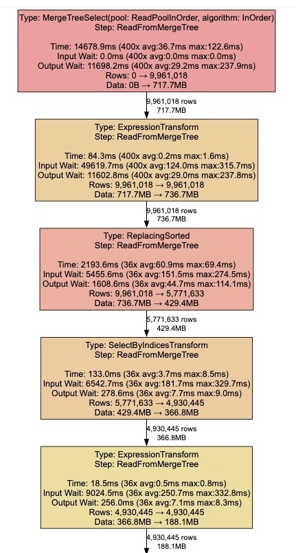
As you can see, there is a 100x reduction in the number of rows and bytes processed. Filtering granules was the win we expected, but there was another we didn’t anticipate. Even when granules are not filtered and unnecessary rows are read from disk, we now filter them before applying the FINAL clause, which has an impact even on small clients.
We finally managed to bring the query time down to ~400ms, from the original 85s. That’s more than a 200x improvement.
Ok But Why
If you’ve read up to this point I can only thank you. Also, you might be wondering why I’m writing this blog.
I’ve spent a few years writing down everything I learned about ClickHouse internals and the process I have followed to investigate and optimize everything I have found in my way. I’m proud of that work, and being unrealistically optimistic, it was useful for others and hopefully will still be. On a more realistic note, I’ve lost (or will lose) access to all that content. Just a few coworkers read it when I originally posted it, and I can’t imagine who is going to read it today.
This is just a small part of what I’ve learned, and sharing it here is a way to try to keep that work alive and accessible for others. Hope it helps.
Footnotes
-
A project can be transferred, a user can change an important attribute, or cancel their subscription, etc. ↩
-
Previous optimizations are still valid but this made it clear that we were under a bit of pressure. ↩
-
I still have to convince myself that this strategy is actually working. We’ll probably change it in the future but so far it’s doing its job. ↩
-
Note that these are tests run on a reduced version of the production data to get intermediate results. That’s why the numbers are noticeably smaller than the ones initially reported. Everything from here to the merges section uses that same reduced dataset. ↩
-
This could have been done at ClickHouse level with a
DEFAULTorMATERIALIZEDcolumn but we preferred to have the logic at application level instead of hidden in a column definition. ↩ -
I pushed a PR to ClickHouse repository to easily measure these steps: PR #108282 ↩
-
There is a line of work already open to make events immutable and work with metric deltas, so we can use materialized views but it’s going to take some time to implement. ↩