SQL Is All You Need
Online gradient descent in ClickHouse
Across all my professional experiences, SQL has been always an important tool. Being it wrestling with Redshift to get historical data to build some models, writing algorithms on Spark to get data from a data lake, or even trying to get dimensional data out of OracleDB.
I strongly believe that our lives would be way easier if SQL was everything (or almost) we needed when it comes to data. In this article, I want to play with the idea of building a machine learning algorithm by just using SQL and ClickHouse. Hence the title, which is a clear reference to the Attention Is All You Need paper.
A bit of context
This piece has been sitting on the back of my head for a while. Since I joined Tinybird one of my responsibilities it’s been to understand the product we are building and help clients to get as much as they can from it. Once I understood ClickHouse’s potential I haven’t managed to prevent myself from thinking about solving problems I had in previous companies.
Although I’m now working as Data Engineer, I’ve spent a vast amount of my career working in roles strongly related to Data Science, and Machine Learning. The two most relevant experiences for this article:
-
Working doing deep learning in a small 3D medical company. There, I heavily contributed in a couple of papers, despite not appearing in them as an author (that was academia and everybody knows how things are played in there, this is another topic that probably deserves a full article for itself)
-
Led the data science efforts in an ad-tech company. Where I implemented a custom version of an online learning algorithm known as FTRL-Proximal in Spark
The common pain in both experiences was always to find a cheap and fast way to store the data that is compatible with real-time inference and also supports experimenting, iterating, and training different models. Being a machine learning practitioner nowadays requires you to use a myriad of tools such as feature stores, training platforms, infrastructure, streams, etc, to be able to train your models and provide batches of predictions.
Now imagine a system being used by a retail company to decide which product to show you based on the probability of you buying it, while they send events to the algorithm to tell it if a shown product has been bought or not. The list of tools needed would keep getting longer.
💭 ClickHouse already has built-in methods implementing linear regression (
stochasticLinearRegression), and logistic regression (stochasticLogisticRegression). Those implementations are a bit rigid but still can be used to build machine learning models without leaving the database in a batch environment.
So let’s play a bit with the idea of building an end-to-end model inside ClickHouse to try to remove all those tools while covering all the described requirements.
To make it easier to follow and reproduce we are going to use some data from the Census Income Data Set:
import pandas as pd

dataset_url = 'https://archive.ics.uci.edu/ml/machine-learning-databases/adult/adult.data'
column_names = ['age', 'workclass', 'fnlwgt', 'education', 'education-num', 'marital-status', 'occupation', 'relationship', 'race', 'sex', 'capital-gain', 'capital-loss', 'hours-per-week', 'native-country', 'y']

df = pd.read_csv(
    dataset_url,
    names = column_names
)
df['y'] = (df['y'] == ' >50K').astype('int')

df.tail()
age workclass fnlwgt education education-num ...
32556 27 Private 257302 Assoc-acdm 12 ... \
32557 40 Private 154374 HS-grad 9 ...
32558 58 Private 151910 HS-grad 9 ...
32559 22 Private 201490 HS-grad 9 ...
32560 52 Self-emp-inc 287927 HS-grad 9 ...
capital-gain capital-loss hours-per-week native-country y
32556 0 0 38 United-States 0
32557 0 0 40 United-States 1
32558 0 0 40 United-States 0
32559 0 0 20 United-States 0
32560 15024 0 40 United-States 1The dataset illustrates a classification problem. It’s quite interesting because it contains continuous and categorical data, something that is not common to see when following implementation examples but that almost every real-life approach will have.
Let’s start by implementing online gradient descent.
Online gradient descent
Online gradient descent is essentially the same as stochastic gradient descent (SGD), the online word is commonly added when applied over stream data. So, instead of randomly selecting a sample from the training set at each iteration, a new iteration is performed every time a new sample is received.
SGD algorithm is easy to describe in pseudo-code:
- Initialize the weights 𝑤
- Iterate over all samples
- For each sample 𝒾 update weights as:
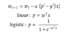
SGD is an iterative method, so having the values of the previous weights, it’s possible to generate the next ones with simple operations. Repeat the process over hundreds/thousands of events and, in theory, it will converge.
Being a recursive algorithm it could probably be implemented using window functions with some recursivity, or recursive CTEs. But leaving apart that they are not supported in ClickHouse, we are interested in a stateful approach (we need the weights to be stored somewhere), and update them every time we receive a new sample. The idea is to use basic database tables and Materialized Views, which are executed on each insert, computing the weights offsets that will later be aggregated. This will allow us to update them on the fly.
First of all, let’s build a simple model using sklearn so we can use it as a reference. It will also allow us to validate results while writing our version. Since this is a classification problem, we’ll use the SGDClassifier with some special settings to simulate online gradient descent. For now, we are going to use only the continuous features and the first 1000 samples, as it will make things easier. Once everything works as expected and things are validated, we will add categorical features, and use the entire dataset if we want.
from sklearn import linear_model

model = linear_model.SGDClassifier(
    loss='log_loss',
    penalty=None,
    fit_intercept=True,
    max_iter=1,
    shuffle=False,
    learning_rate='constant',
    eta0=0.01
)

X = df[['age', 'fnlwgt', 'education-num', 'capital-gain', 'capital-loss', 'hours-per-week']]
y = df[['y']]
model = model.fit(X[:1000], y[:1000])

print(model.intercept_[0])
print(dict(zip(X.columns, model.coef_[0])))
0.10499999999999998
{'age': 16.665000000000006,
'capital-gain': 2844.8600000000006,
'capital-loss': 253.21000000000004,
'education-num': 4.035000000000002,
'fnlwgt': 2824.270000000001,
'hours-per-week': 14.259999999999996}And this is the SQL implementation:
DROP DATABASE IF EXISTS sgd SYNC;
CREATE DATABASE sgd;

CREATE TABLE sgd.samples (
    age UInt8,
    workclass LowCardinality(String),
    fnlwgt UInt32,
    education LowCardinality(String),
    educationNum UInt8,
    maritalStatus LowCardinality(String),
    occupation LowCardinality(String),
    relationship LowCardinality(String),
    race LowCardinality(String),
    sex LowCardinality(String),
    capitalGain UInt32,
    capitalLoss UInt32,
    hoursPerWeek UInt32,
    nativeCountry LowCardinality(String),
    income LowCardinality(String),
    dt DateTime DEFAULT now()
)
ENGINE = MergeTree
ORDER BY dt;

CREATE TABLE sgd.weights (
    column String,
    w Float64
)
ENGINE = SummingMergeTree
ORDER BY column;

CREATE MATERIALIZED VIEW sgd.update_weights TO sgd.weights AS (
    WITH sum(x * w0) OVER () AS wTx
    SELECT
        column,
        - 0.01 * (1/(1+exp(-wTx)) - y) * x as w
    FROM (
        SELECT
            dt,
            key column,
            value x,
            y
        FROM
        (
            SELECT
                dt,
                income = '>50K' y,
                ['intercept', 'age', 'fnlwgt', 'educationNum', 'capitalGain', 'capitalLoss', 'hoursPerWeek'] keys,
                [1, age, fnlwgt, educationNum, capitalGain, capitalLoss, hoursPerWeek] values
            FROM sgd.samples
        )
        ARRAY JOIN
            keys AS key,
            values AS value
    )
    ANY LEFT JOIN (
        SELECT column, w w0 FROM sgd.weights FINAL
    ) USING column
);
After ingesting the first 1000 samples 1-by-1 into sgd.samples this is the result we are getting:
SELECT
    column,
    w
FROM sgd.weights
FINAL
ORDER BY column ASC| column | w |
|---|---|
| age | 16.665000000000006 |
| capitalGain | 2844.8600000000006 |
| capitalLoss | 253.21000000000004 |
| educationNum | 4.035000000000002 |
| fnlwgt | 2824.270000000001 |
| hoursPerWeek | 14.259999999999996 |
| intercept | 0.10499999999999998 |
Everything is looking fine, the results are the same as we got by running sklearn! Honestly, I was expecting some minor differences here but I’m not going to complain.
At this point, if you are familiar with ClickHouse you’ll realize that ingesting row by row is suboptimal. The good news is that it’s usually also suboptimal for gradient descent, and there are already solutions out there.
Mini batches
Stochastic gradient descent with mini-batches is essentially the same but instead of going sample by sample, a batch of N samples is processed in each step. The algorithm described in pseudo-code is basically:
- Initialize the weights 𝑤
- Iterate over all samples in batches of size b:
- For each batch update weights as:
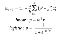
So, in plain English, exactly the same as before but the update step is the average over the entire mini-batch. If you are interested in reading more about the differences and when to use each one there are good resources out there, listing a few of them:
- The difference between Batch Gradient Descent and Stochastic Gradient Descent
- Differences Between Gradient, Stochastic and Mini Batch Gradient Descent
- Mini Batch Gradient Descent
- Understanding Mini-Batch Gradient Descent
We can add mini-batches by slightly modifying the previous SGD implementation:
DROP DATABASE IF EXISTS sgd SYNC;
CREATE DATABASE sgd;

CREATE TABLE sgd.samples (
    age UInt8,
    workclass LowCardinality(String),
    fnlwgt UInt32,
    education LowCardinality(String),
    educationNum UInt8,
    maritalStatus LowCardinality(String),
    occupation LowCardinality(String),
    relationship LowCardinality(String),
    race LowCardinality(String),
    sex LowCardinality(String),
    capitalGain UInt32,
    capitalLoss UInt32,
    hoursPerWeek UInt32,
    nativeCountry LowCardinality(String),
    income LowCardinality(String),
    dt DateTime DEFAULT now()
)
ENGINE = MergeTree
ORDER BY dt;

CREATE TABLE sgd.weights (
    column String,
    w Float64
)
ENGINE = SummingMergeTree
ORDER BY column;

CREATE MATERIALIZED VIEW sgd.update_weights TO sgd.weights AS (
    WITH
        sum(x * w0) OVER (partition by dt) AS wTx,
        countDistinct(dt) OVER () AS b
    SELECT
        column,
        - (0.01/b) * (1/(1+exp(-wTx)) - y) * x as w
    FROM (
        SELECT
            dt,
            key column,
            value x,
            y
        FROM
        (
            SELECT
                dt,
                income = '>50K' y,
                ['intercept', 'age', 'fnlwgt', 'educationNum', 'capitalGain', 'capitalLoss', 'hoursPerWeek'] keys,
                [1, age, fnlwgt, educationNum, capitalGain, capitalLoss, hoursPerWeek] values
            FROM sgd.samples
        )
        ARRAY JOIN
            keys AS key,
            values AS value
    )
    ANY LEFT JOIN (
        SELECT column, w w0 FROM sgd.weights FINAL
    ) USING column
);
Finally, after running it with mini-batch = 5, meaning ingesting 5 rows each time, we get the following weights:
SELECT
    column,
    w
FROM sgd.weights
FINAL
ORDER BY column ASC| column | w |
|---|---|
| age | 15.909999999999995 |
| capitalGain | 2868.7700000000013 |
| capitalLoss | 165.49 |
| educationNum | 4.204999999999998 |
| fnlwgt | 341.324999999998 |
| hoursPerWeek | 13.735000000000003 |
| intercept | 0.04499999999999994 |
Note that the SQL code is also prepared to receive a flexible mini-batch size, so an arbitrary number of rows can be ingested every time. This will be extremely useful in case you are receiving data from a stream that is buffering events together, and flushing every certain seconds.
The only missing step now is to add categorical features. This will require using one-hot encoder in sklearn, but in our code is just a matter of changing the subquery that is pivoting the data, from:
SELECT
    dt,
    key column,
    value x,
    y
FROM
(
    SELECT
        dt,
        income = '>50K' y,
        ['intercept', 'age', 'fnlwgt', 'educationNum', 'capitalGain', 'capitalLoss', 'hoursPerWeek'] keys,
        [1, age, fnlwgt, educationNum, capitalGain, capitalLoss, hoursPerWeek] values
    FROM sgd.samples
)
ARRAY JOIN
    keys AS key,
    values AS value
To something like this:
SELECT
    dt,
    key column,
    value x,
    y
FROM
(
    SELECT
        dt,
        income = '>50K' y,
        [
            'intercept',
            'age',
            'fnlwgt',
            'educationNum',
            'capitalGain',
            'capitalLoss',
            'hoursPerWeek',
            'workclass:' || workclass,
            'education:' || education,
            'maritalStatus:' || maritalStatus,
            'occupation:' || occupation,
            'relationship:' || relationship,
            'race:' || race,
            'sex:' || sex,
            'nativeCountry:' || nativeCountry
        ] keys,
        [
            1,
            age,
            fnlwgt,
            educationNum,
            capitalGain,
            capitalLoss,
            hoursPerWeek,
            1,
            1,
            1,
            1,
            1,
            1,
            1,
            1
        ] values
    FROM sgd.samples
)
ARRAY JOIN
    keys AS key,
    values AS value
After repeating the process weights will be looking as
SELECT
    column,
    w
FROM sgd.weights
FINAL
ORDER BY column ASC| column | w |
|---|---|
| age | 6.489999999999998 |
| capitalGain | 926.0200000000001 |
| capitalLoss | 107.03 |
| education:10th | -0.02 |
| education:11th | -0.065 |
| education:12th | 0.01 |
| … | … |
| education:Masters | 0.05 |
| education:Prof-school | 0.03 |
| education:Some-college | 0.035 |
| educationNum | 1.259999999999999 |
| fnlwgt | -361.92500000000473 |
| hoursPerWeek | 3.579999999999996 |
| intercept | -0.0050000000000000565 |
| maritalStatus:Divorced | -0.09500000000000003 |
| maritalStatus:Married-AF-spouse | -0.01 |
| … | … |
| maritalStatus:Widowed | -0.01 |
| nativeCountry:? | 0.005000000000000001 |
| nativeCountry:Cambodia | 0.01 |
| … | … |
| nativeCountry:Thailand | 0.01 |
| nativeCountry:United-States | -0.009999999999999943 |
| occupation:? | -0.02 |
| occupation:Adm-clerical | -0.03 |
| … | … |
| workclass:? | -0.02 |
| workclass:Federal-gov | 0.019999999999999997 |
| workclass:Local-gov | 0.009999999999999998 |
| workclass:Private | -0.11 |
| workclass:Self-emp-inc | 0.05 |
| workclass:Self-emp-not-inc | 0.025 |
| workclass:State-gov | 0.019999999999999997 |
Finally, to run a prediction we just have to run a query to retrieve the weights and apply the simple computations:
WITH
    sum(x * w0) OVER (partition by dt) AS wTx
SELECT
    1/(1+exp(-wTx)) AS p
FROM (
    SELECT
        dt,
        key column,
        value x
    FROM
    (
        SELECT
            now() dt,
            [
                'intercept',
                'age',
                'fnlwgt',
                'educationNum',
                'capitalGain',
                'capitalLoss',
                'hoursPerWeek',
                'workclass:' || workclass,
                'education:' || education,
                'maritalStatus:' || maritalStatus,
                'occupation:' || occupation,
                'relationship:' || relationship,
                'race:' || race,
                'sex:' || sex,
                'nativeCountry:' || nativeCountry
            ] keys,
            [
                1,
                age,
                fnlwgt,
                educationNum,
                capitalGain,
                capitalLoss,
                hoursPerWeek,
                1,
                1,
                1,
                1,
                1,
                1,
                1,
                1
            ] values
        FROM (
             SELECT
                20 age,
                'Private' workclass,
                148294 fnlwgt,
                'Some-college' education,
                10 educationNum,
                'Never-married' maritalStatus,
                'Other-service' occupation,
                'Own-child' relationship,
                'White' race,
                'Male' sex,
                0 capitalGain,
                0 capitalLoss,
                40 hoursPerWeek,
                'United-States' nativeCountry
        )
    )
    ARRAY JOIN
        keys AS key,
        values AS value
        )
ANY LEFT JOIN (
    SELECT column, w w0 FROM sgd.weights FINAL
) USING column
LIMIT 1
Conclusion
It’s possible to implement logistic regression in SQL, and thanks to ClickHouse and the Materialized Views we have managed to implement an online gradient descent algorithm capable of predicting events in real-time. This opens the door to a lot of possibilities.
Going back to the original example, the one about a retail company that wants to decide in real-time which product to show to a client based on the probability of buying them. We’d have to program the described algorithm in your database, build an easy way to ingest data in real-time from the online store to instantly update your model, and then provide an interface to run inference and return probabilities.
Lucky us, we don’t have to do that much! We already implemented the algorithm, and the interfaces to ingest and query data already come with the database.
Of course, the approach described here is simple, SGD is not the strongest model out there, but it’s doing its job and setting a good baseline. Perhaps you are not confident enough with SQL but I hope this post encourages others to run similar experiments, trying to get as much as they can from their day-to-day tools.